In the posts Quantifying Market Risk and Quantifying Trading System Risk we had a look at the risks involved in the financial markets in general and the risks involved in a quantitative investment approach in particular. Let’s now have a look at these two together. Furthermore, let’s have a look at how they apply to a quantitative investment in the futures markets. To illustrate the risks involved we will use the current Quantopolis Investment Strategies as summarized below:
| Strategy | ROC | MAX DD | RR | Capital |
| TF Pullback | 63.16% | -59.92% | 1.05 | $9,250 |
| VX Short | 65.98% | -29.65% | 2.22 | $14,500 |
| ZN Long | 51.35% | -82.54% | 0.62 | $8,000 |
| ES Pullback | 64.68% | -56.39% | 1.15 | $13,325 |
| NQ Pullback I | 57.15% | -61.74% | 0.93 | $15,250 |
| NQ Pullback II | 79.90% | -64.50% | 1.24 | $16,350 |
| Portfolio I | 52.75% | -20.11% | 2.62 | $27,825 |
| Portfolio II | 39.32% | -17.05% | 2.31 | $76,675 |
The above table shows the expected Return on Capital, Maximum Drawdown, Risk Reward and Minimum Allocated Capital for each strategy. These numbers are based on the historical backtesting observations for each strategy.
Quantifying Strategy Risk
The minimum allocated capital for each of the strategies listed above is calculated as the margin requirement for the underlying market plus the maximum historical drawdown during the backtesting. As discussed in the post Quantifying Trading System Risk there is no guarantee that future drawdowns are going to be less than or equal to those observed in the past.
In Quantifying Trading System Risk we used mathematics and statistics to calculate the amount of capital required such that we can say with more than 95% confidence or with more than 99% confidence that we are not going to go bust when putting our monies in a particular investment strategy. Applying this methodology to the above strategies we get the following results:
| Strategy | Historical |
95% | 99% |
| TF Pullback | $9,250 | $13,500 | $19,000 |
| VX Short | $14,500 | $16,000 | $19,500 |
| ZN Long | $8,000 | $4,500 | $6,000 |
| ES Pullback | $13,325 | $11,500 | $14,500 |
| NQ Pullback I | $15,250 | $24,000 | $35,000 |
| NQ Pullback II | $16,350 | $22,000 | $31,000 |
| Portfolio I | $27,825 | $20,000 | $22,000 |
| Portfolio II | $76,675 | $41,000 | $46,000 |
The above table shows the amount of capital required such that we can be at least 95% confident or 99% confident that we are not going to go bust when investing monies in the above strategies. Looking at the above numbers we see that in some cases the historical capital requirement is below the 95% confidence level and in other cases it is above the 95% confidence level.
While the historical capital requirement looks at the worst historical case scenario as defined by the maximum historical drawdown, as discussed in more detail in the post Quantifying Trading System Risk, the mathematical approach looks at the probability of having similar or larger drawdowns in the future. This is done by considering the average wins and losses for each strategy as well as the probability of winning or loosing. Thus the probabilistic approach gives a more complete picture of what can be expected in the future.
As discussed in the post Quantifying Trading System Risk, the probability of going bust is highest at the onset. This is because as the investment starts to generate positive returns, if all the capital is retained within the system, the system can withstand even larger drawdowns before going bust. Thus the probability of going bust goes down over time for a money making system.
Before we move on, it is very important to emphasize here that the above numbers have meaning only if the underlying strategies are robust. As discussed in Buyer Beware the great majority of quantitative strategies out there are no good. Thus any results or probabilities for these strategies are nothing more than castles in the air.
Moving Forward
The above numbers are based on current values for the underlying markets. For markets such as the stock indices and treasuries which tend to go up over time, these numbers will have to be adjusted accordingly. This is because as the index goes up, although the relative drawdown might stay the same, the absolute drawdown (or points) will also go up and hence the required capital will need to be greater. On the flip side, if the market value has gone up, then the absolute returns will also go up. Thus, since both drawdowns and returns go up, the expected return on capital as well as the risk reward ratio stay the same.
For example, looking at the Nasdaq 100 Index:
In 2013 the NDX and the corresponding NQ futures were around 3,500. Thus a 1% change is 35 points or $700.
In 2018 the NDX and the corresponding NQ futures hit 7,000 for the first time. Thus a 1% change is 70 points or $1,400.
In addition to the price of the contract changing over time, margin requirements can also change from time to time. For example current margin requirements for the VX futures are at $9,900 per contract. However, looking at the historical data, they have been as low as $2,250 and as high as $13,200. Thus, the 99% capital requirement for the VX Short strategy would have to be adjusted to $27,300 to account for the possibility of a higher margin requirement.
The Portfolio Approach
Looking at the above table we see that for each level of confidence, the amount of capital required for Portfolio I and Portfolio II is less than the sum of the capital required for the individual strategies that are traded in the portfolio. The computation of the portfolio capital as the simple addition of the capital requirement of its constituent strategies assumes that all strategies are going to hit their maximum drawdown at the same time. This situation is an extreme case and thus overstates the amount of capital required.
By using a probabilistic approach and looking at the trades as part of a portfolio, we can get a better estimate of the capital required when trading the strategies together as a portfolio. This is a clear advantage of true diversification. By using different strategies with different assumptions, one can minimize the risk thereby increasing the potential return on capital.
Quantifying Market Risk
The other type of risk inherent to a quantitative investment in the futures markets is general market risk. This is due to adverse news events around the world and their effects on the financial markets.
In the post Quantifying Market Risk we used statistics to quantify the probability of a severe adverse effect occurring and determined that we could say with more than 99% confidence that the DJIA will not move by more than 3.25% in one day. Although other stock indices such as the NASDAQ might move more than the DJIA, it is reasonable to extrapolate this statement for the DJIA to other stock indices. Thus we can make a general statement and say with confidence that the probability for an extreme move in the stock indices is less than 1%.
The above statement assumes that we are in the market all the time. However, this is not the case for many quantitative investment strategies. In fact, as summarized on the Investment Strategies page, the Quantopolis strategies spend most of the time in cash with no open positions.
| Strategy | Trades | Hold |
Exposure |
| TF Pullback | 9 | 3.64 | 0.13 |
| VX Short | 15 | 16.67 | 1 |
| ZN Long | 12 | 20.8 | 1 |
| ES Pullback | 10 | 1.75 | 0.07 |
| NQ Pullback I | 11 | 3.43 | 0.15 |
| NQ Pullback II | 18 | 3.34 | 0.24 |
| Portfolio I | 25 | 10.7 | 0.54 |
| Portfolio II | 75 | 8.64 | 0.43 |
The above table shows the average number of trades per year and the average holding period per trade for each strategy. The exposure column shows the average yearly exposure for each strategy. Thus for example, looking at the ES Pullback which has on average about 10 trades a year each with an average holding period of 1.75 days, the average number of days it has an open position is 17.5 days per year. Since there are approximately 250 trading days a year, the average yearly exposure for the ES Pullback is 0.07.
Thus if the probability of an adverse market effect is less than 1% and the probability of being in the market is 7%, then the probability of experiencing an adverse market effect when has an open position is less than 0.07%.
So, Are These Investments Risky?
Combining the results from the above paragraphs we see that the possibility of losing money due to the strategy performing badly or experiencing an adverse market effect when holding an open position is very small. In particular, statistics shows us that the likelihood of failure is less than 1%.
To my mind this probability is small enough and the potential rewards are big enough that a quantitative investment in the futures markets is worth pursuing. This is the reason why I have my own monies in these strategies and why I feel comfortable making them available to others as well. That said, as discussed in the Legal Disclaimer, every individual must do their own due diligence and make their own decision as to whether such an investment is suitable for them.
Insurance For a Rainy Day
As discussed above the risks involved are small enough and the potential rewards significant enough that a quantitative investment approach in the futures markets as described above is appealing to many an investor. That said, one can take additional steps to further mitigate their portfolio against adverse events. This can be done by purchasing insurance in the form of options contracts.
Option contracts are also a derivative instrument and they offer the investor a lot of flexibility including the opportunity to purchase protection for their portfolio and hedge themselves against adverse market conditions. As an example, let’s have a look at the ES Pullback strategy.
The ES Pullback strategy trades the ES futures which are related to the S&P 500. In particular, this strategy is a value based strategy and enters the market when it perceives the market to be cheap on a short term basis. In other words, this strategy buys the market when prices have fallen with the hope of selling out and closing the position when the market recovers. This implies that this strategy will take a loss if the market continues to fall. As discussed above, in more than 99% of the time this is just business as usual and the strategy will take a loss and wait for the next opportunity.
If one wants to attempt to minimize this risk even further then one can look into buying an out of the money put option on the S&P 500 every time one has an open position in the ES Pullback. Like any other insurance product, this comes at a cost. However for a small ongoing cost, the investor can achieve protection in the very unlikely event of a catastrophic loss.
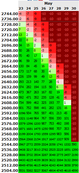
For example, at the time of this writing the S&P 500 closed at 2,733.99 and the ES Futures June contract at 2,730. Say the ES Pullback strategy had a buy signal today and the investor bought one contract of the ES June futures at 2,730. For an additional $10 plus the costs of commissions etc.. the investor can also buy a May 29th put option on the S&P 500 with a $2,550 strike price.
If the market rallies and the futures contract goes up, then the investor makes the money they would have made before less the $10 + trade costs he or she spent buying the option contract. On the other hand if the if the futures contract dropped by 10% or 20% the gain in the options contract would offset any losses from the futures contract.
The beneficial effect of the out of the money put option becomes more significant as the prices drop hard. This would be the case of a catastrophic black swan event. The following table summarizes the profit and loss for different market movements:
| Price | Change | Futures | Option | Total |
| 2757.30 | 1% | $1,365 | -$10 | $1,355 |
| 2702.70 | -1% | -$1,365 | $22 | -$1,343 |
| 2593.50 | -5% | -$6,825 | $1,096 | -$5,729 |
| 2457.00 | -10% | -$13,650 | $9,213 | -$4,437 |
| 2184.00 | -20% | -$27,300 | $36,500 | $9,200 |
This table shows that using a put option contract offers great protection in the case of catastrophic events. Not only does it reduce losses in strong down market events, but it also has the potential of turning an oversized loss into a gain in the event of a catastrophic market event. In addition it limits the maximum loss of the strategy in sudden downturns to less than $6,000 which is well within the limit of the maximum drawdown and the confines of the capital requirements for the strategy. Furthermore, since the ES Pullback averages only about 10 trades per year and has an expected average annual return of $13,325, buying a $10 option contract with each trade would only decrease the expected average annual return to $13,225. Thus it is a very doable approach to risk mitigation even if the price of the put is higher than $10.